


Abstract
The Interstellar Boundary Explorer (IBEX) mission has shown that variations in the energetic neutral atom (ENA) flux from the outer heliosphere are associated with the solar cycle and longer-term variations in the solar wind (SW). In particular, there is a good correlation between the dynamic pressure of the outbound SW and variations in the later-observed IBEX ENA flux. The time difference between observations of the outbound SW and the heliospheric ENAs with which they correlate ranges from approximately 2 to 6 yr or more, depending on ENA energy and look direction. This time difference can be used as a means of "sounding" the heliosheath, that is, finding the average distance to the ENA source region in a particular direction. We apply this method to build a 3D map of the heliosphere. We use IBEX ENA data collected over a complete solar cycle, from 2009 through 2019, corrected for survival probability to the inner heliosphere. Here we divide the data into 56 "macropixels" covering the entire sky. As each point in the sky is sampled once every 6 months, this gives us a time series of 22 points macropixel–1 on which to time-correlate. Consistent with prior studies and heliospheric models, we find that the shortest distance to the heliopause, dHP, is slightly south of the nose direction (dHP ∼ 110–120 au), with a flaring toward the flanks and poles (dHP ∼ 160–180 au). The heliosphere extends at least ∼350 au tailward, which is the distance limit of the technique.
Export citation and abstract BibTeX RIS
1. Introduction
When Voyager 1 crossed the termination shock (TS) in 2004 at a distance of 94 au from the Sun, we obtained our first definitive measurement of the scale of the heliosphere (Stone et al. 2005). The Voyagers have continued to survey the dimensions of the upwind heliosphere, with the subsequent TS crossing of Voyager 2 in 2007 at 84 au (Stone et al. 2008) and the Voyager 1 and 2 crossings of the heliopause (HP) in 2012 at 122 au (Stone et al. 2013) and 2018 at 119 au (Stone et al. 2019), respectively. These in situ measurements have provided the necessary ground truth as to the scale of the heliosphere, but as such, we only have direct measurements along two spacecraft trajectories at specific instances in time, providing important but very spatially and temporally limited information about the dimensions of the heliosphere.
With the launch of the Interstellar Boundary Explorer (IBEX) in 2008 (McComas et al. 2009a), it has become possible to map the dimensions of the heliosphere remotely. Observations of energetic neutral atoms (ENAs) from the outer heliosphere have shown that variations in the ENA flux are associated with the solar cycle and even longer-term variations in the solar wind (SW) output. In particular, there is a good correlation between the dynamic pressure of the outbound SW and variations in the IBEX ENA flux observed 2–4 yr later for the upwind hemisphere and even longer in the downwind direction (Reisenfeld et al. 2016; McComas et al. 2017, 2019a, 2020). From this, one can derive the distance to the ENA source region. For much of the sky, the observed ENA flux, often referred to as the globally distributed flux (GDF; McComas et al. 2009b), originates in the heliosheath (HS), the region between the TS and the HP. Thus, by determining the time lag between an outgoing SW pressure disturbance observed at 1 au and a correlated signature in the ENA flux, one can determine the distance to the average emission distances within the HS. We refer to this technique as "sounding" the distance, in direct analogy with underwater sonar, and we call the time lag the "trace-back" time, ttb (Reisenfeld et al. 2012, 2016).
The sounding method was first applied early in the IBEX mission by Reisenfeld et al. (2012) in the direction of the ecliptic poles. The poles have the advantage of being observed nearly continuously by IBEX, in contrast to other parts of the sky, which are observed only once every 6 months. This first study, which made use of the first 2 yr of 0.5–6.0 keV ENA observations from the IBEX-Hi instrument (Funsten et al. 2009a), suggested a distance to the HP of 215 au in the direction of the ecliptic north pole and 165 au toward the south pole. The analysis was done again by Reisenfeld et al. (2016) using a total of 7 yr of IBEX-Hi data, arriving at HP distances of 220 au for the north ecliptic pole and 190 au for the south. Based on modeling work by Zirnstein et al. (2018), it was recognized that the relation used by Reisenfeld et al. (2012, 2016) for the trace-back time would overestimate distances to the HP and needed to be adjusted. Thus, a new analysis was performed by Reisenfeld et al. (2019) using the revised relation for ttb, arriving at HP distances of 160 au in the direction of the north ecliptic pole and 150 au in the south.
Galli et al. (2016) also utilized ENA observations to estimate the dimensions of the heliosphere using a different method. They used 0.015–2 keV ENA observations from the IBEX-Lo instrument (Fuselier et al. 2009) to estimate the thickness of the ENA source region in the downwind hemisphere. They computed the line-of-sight (LOS) integrated plasma pressure in the HS, Δ P•L, from ENA flux measurements and then compared this to modeled values for the plasma pressure in the HS to arrive at an ENA source thickness of 220 ± 110 au. The error bars are rather large because of the statistical uncertainties in the IBEX-Lo observations and because they do not take into account contributions to the LOS-integrated pressure above 2 keV.
It is worth pointing out here that studies that use ENA observations to constrain the thickness of the HS, including ours, will at least somewhat underestimate the distance to the HP. Energetic ions in the HS experience charge exchange with interstellar neutrals, effectively "cooling" the plasma and limiting the distance at which we can view the heliosphere using ENAs, particularly in the downwind direction. This is much less of a concern in the upwind hemisphere, as the plasma cooling length is considerably longer than the expected distances to the HP.
A different approach to determine the global size of the heliosphere was taken by McComas et al. (2019b), who used combined observations by the Voyagers and IBEX to estimate the size and location of the TS. These authors approximated the TS as a sphere and determined its size and the offset of its center from the Sun. In addition to the Voyager TS crossings, they identified two additional points on the TS by marking the locations where Voyagers 1 and 2 magnetically disconnect from the anomalous cosmic-ray (ACR) source, presumed to be the TS boundary. Because of the bluntness of the TS in the upwind direction, the two respective disconnection points trace back along the HS magnetic field to points where the field has just disconnected from the TS at its tailward extreme. These four points can be fit to a sphere having a radius of 117 au and a center offset by 32 au downwind, 27 au to the north, and 12 au to the port side of the heliosphere (as viewed looking upwind from the Sun). Their results yielded a TS that is closer to the Sun south of the nose and on the starboard side of the HS, in qualitative agreement with IBEX observations (McComas et al. 2020).
The present study returns to the sounding method but now applies it to the full sky for the purpose of mapping out the global shape of the HP and creating, for the first time, an empirical 3D map of the heliosphere. By the end of 2019, IBEX had completed an 11 yr survey of heliospheric ENA emissions, resulting in 22 sky maps collected over consecutive 6 month intervals (McComas et al. 2020). Thus, in any direction, it is possible to time-correlate the ENA flux with the SW dynamic pressure using a 22 point time series. Furthermore, 11 yr of ENA observations means we have a complete solar cycle of measurements, which should allow for stronger constraints on the time correlations.
IBEX also observes another ENA signal, an enhancement of ENAs forming a nearly circular ribbon across the sky, unanticipated prior to IBEX (McComas et al. 2009b; Funsten et al. 2013). The ribbon is centered ∼8° from the direction of the local interstellar magnetic field (LISMF) (Funsten et al. 2009b; Schwadron et al. 2009; Zirnstein et al. 2016) and is widely believed to be formed from secondary ENAs produced in the draped LISMF region outside the HP by charge exchange between pickup ions from the neutralized supersonic SW and interstellar neutral atoms (e.g., McComas et al. 2009b; Heerikhuisen et al. 2010; Zirnstein et al. 2015, 2019). The center of the ribbon lies near the B–V plane of the heliosphere (the plane defined by the LISMF direction (B) and the interstellar flow direction (V)), as well as the hydrogen deflection plane (the plane defined by the primary interstellar He and the interstellar H flow directions; Lallement et al. 2010; Schwadron et al. 2018). If the ribbon ENAs indeed originate beyond the HP, they are not part of the GDF; therefore, to accurately apply the sounding method, one must either avoid parts of the sky where the GDF and the ribbon emissions are combined in the LOS integral or separate the ribbon flux from the GDF and analyze the populations independently. In this study, we choose the latter approach.
In Section 2, we describe the IBEX ENA observations used in this study and discuss the method for separating the GDF from the ribbon flux in order to isolate only the ENA flux from the HS. In Section 3, we describe the sounding method and how it is applied to determine the distance to the ENA source regions in all directions, and in Section 4, we present the resulting 3D structure of the HP using three different assumed shapes for the TS. We also discuss how the derived shape of the HP compares to expectations from simulations and how the derived HP distances compare to "ground truth," the actual HP crossing distance of Voyagers 1 and 2. Section 5 summarizes our results.
2. Observations and Data Preparation
2.1. Data Selection
For this study, we utilize the first 11 yr of IBEX-Hi ENA flux measurements from the five energy passbands centered on 0.71, 1.11, 1.74, 2.73, and 4.29 keV (these are also referred to ESA steps 2–6). The IBEX spacecraft maintains a nearly Sun-pointed spin axis, repointing in ecliptic longitude back toward the Sun every ∼7.5 days during the period between launch and an orbit-stabilizing maneuver in 2011 and then every ∼4.5 days thereafter (McComas et al. 2011, 2012). As IBEX spins, it samples a fixed longitudinal swath of the sky over all latitudes. Each repointing shifts the longitude by 4°–5° to sample the next adjacent swath. Over the course of 6 months, the spin axis rotates through 180° to produce a complete all-sky map. Because of the ∼30 km s−1 motion of the Earth (and therefore IBEX) around the Sun, half of the data in a 6 month map is collected over the half spin when the IBEX spacecraft is moving toward the incoming observed ENAs (Ram data), and half is taken over the half spin when it is moving away from them (anti-Ram data). In the following 6 months, another all-sky map is collected, but now the portion of the sky that was previously sampled in the Ram direction is sampled in the anti-Ram direction, and vice versa.
A consequence of the alternate Ram/anti-Ram sampling is that a given region appears considerably brighter when observed in the Ram direction than when observed in the anti-Ram direction, complicating direct comparison. Therefore, time variation studies often make use of yearly maps, where the Ram portions of two adjacent 6 month maps are combined, resulting in "Ram-only" maps. Similarly, yearly "anti-Ram-only" maps can be constructed. Such maps allow for the most directly comparable measurements of time variation of the whole sky (McComas et al. 2012, 2014, 2017, 2020).
Here we take a different approach in order to maximize the time resolution for applying the sounding method. Specifically, we use 6 month map sets where the ENA fluxes have been Compton–Getting (CG) corrected by transforming the data from the spacecraft frame to the solar inertial frame (McComas et al. 2010). The direct CG correction transforms both the flux and the measurement energies from the spacecraft frame to a solar inertial frame. Because the transformed energies depend on the look angle of the IBEX-Hi sensor relative to the spacecraft velocity vector, the measurement energies in a CG-corrected map vary across the map. We prefer to work with maps having the same measurement energy for all of the pixels; thus, for a given passband, a "monoenergetic" map is created, consisting of fluxes shifted from the direct CG-transformed values to values at a common solar inertial frame energy. For convenience, the energies assigned to the monoenergetic CG maps correspond to the original spacecraft-frame central energy values for each of the passbands. The ENA fluxes are also adjusted for the survival probability of ENAs traveling 100 au from beyond the TS to 1 au (Bzowski 2008) so that they reflect the expected ENA flux levels in the HS. All data used in this study are taken from the latest and most complete release of the IBEX-Hi data (McComas et al. 2020), which incorporated all of these corrections.
2.2. Ribbon Separation
As mentioned in the Introduction, applying the sounding method to regions of the sky containing the ENA ribbon is complicated by the fact that IBEX is observing ENAs from two distinct sources, as the GDF originates in the HS and the ribbon emissions are likely coming from the outer HS, beyond the HP. Thus, to apply the sounding method for mapping out the boundaries of the heliosphere, one must either ignore the regions of the sky containing the ribbon altogether or separate and remove the ribbon flux. Because so much of the sky is covered by the ribbon, we have decided to take the ribbon separation and removal approach. A ribbon separation technique introduced by Schwadron et al. (2011) Requires summing multiple maps together to get good enough statistics to accurately identify ribbon versus GDF flux at the level of individual 6° × 6° pixels. Because we wish to carry out ribbon separation on individual 6 month maps in order to preserve as much time resolution as possible, we have devised a different technique.
We summarize the technique here and describe the procedure in detail in the Appendix. We transform the ecliptic-frame ENA maps described above into a "ribbon-centered" frame, where the ribbon center is located at the "north pole" of the maps and the ribbon itself appears as a constant latitude feature centered on a latitude 75° from the pole. In this manner, it is easy to take longitudinal cuts across the ribbon and fit functions approximating the shape of the ribbon and the GDF in order to partition the ribbon flux from GDF. To improve statistics, prior to fitting, we average the flux in longitude every 24° (4 pixels), resulting in 15 longitude strips, each with 30 6° wide bins spanning pole-to-pole.
For each of these strips, we identify a set of latitude bins on either side of the ribbon (but not including it) and fit a second-order polynomial to capture the shape of the GDF beneath the ribbon. The flux associated with this fit is subtracted from the total flux in the ribbon bins, and a Gaussian representing the cross-sectional shape of the ribbon is fit to the remaining flux. For each bin in the ribbon, we ratio the Gaussian fit to the sum of the Gaussian and second-order polynomial fits and use this ratio to partition the total observed flux in the bin between the ribbon and the GDF. For a given latitude, the same ratio is applied to each of the four initial 6° × 6° ribbon-centered pixels composing a bin. What results are two maps, one of the GDF and one of the ribbon flux. The separated maps are then transformed back into the ecliptic frame. Figure 1 gives an example of the separation technique applied to the 2013B maps. See the Appendix for further discussion.
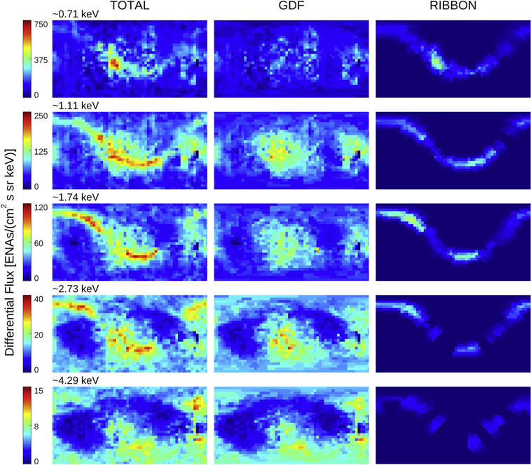
Figure 1. The 2013B ENA maps, showing the ribbon separation method. The left column shows the original 6 month, CG- and survival probability–corrected maps for the five IBEX-Hi energy passbands. The middle and right columns show the corresponding GDF and ribbon-only maps, respectively. The GDF maps are used to derive the HS fluxes for use in the sounding method. See the Appendix for details on the ribbon separation technique.
Download figure:
Standard image High-resolution imageThe GDF maps in Figure 1 show that our technique successfully removes the ribbon. The pressure enhancement associated with the heliospheric nose appears as a nearly circular structure centered ∼20° south of the upwind direction, owing to the asymmetric pressure of the external interstellar magnetic field (ISMF) draped around the heliosphere (McComas & Schwadron 2014). The enhancement associated with flux coming from the tailward direction appears at the edges of the maps (McComas et al. 2013). For this study, we are not concerned with the ribbon maps, although one could apply the sounding method to these as well to find the distance to the ribbon, which will be the focus of a future study. We acknowledge that applying our ribbon separation technique to 24° wide strips and then using the result to partition fluxes in individual 6° × 6° pixels leads to an under- or oversubtraction of the ribbon flux in a given pixel. However, as we shall see in the next section, the sounding method will be applied to groups of summed 6° × 6° pixels, or "macropixels" (again, to improve statistics); thus, the partitioning error present at the native pixel scale will average out.
2.3. Binning of Data into Macropixels
Before applying the sounding method to the ENA data, we divide the sky into 56 regions, or macropixels, of roughly the same solid angle of roughly a quarter steradian each. We select macropixels that are large enough to reduce the statistical noise within a pixel to a level where statistics do not significantly influence the time correlation but small enough to capture a reasonable spatial resolution. Figure 2 shows an overlay of the boundaries of the 56 macropixels on a representative ENA map for context. The sky is divided into seven latitude bands of macropixels, which we will respectively refer to as the equatorial pixels (12 pixels between 15°N and 15°S), the north and south midlatitude pixels (12 pixels each spanning 15°N–45°N and 15°S–45°S), the north and south high-latitude pixels (9 pixels each spanning 45°N–80°N and 45°S–80°S), and 2 polar pixels (each extending from 80°N/S to the poles). In longitude, the macropixels are oriented such that the longitude of the heliospheric upwind direction (−105°, 5°) is aligned with the center of a macropixel, which we refer to as the nose pixel. The Voyager 1 and 2 locations are also shown and are located near the centers of two macropixels, which we refer to as the V1 and V2 pixels, respectively.
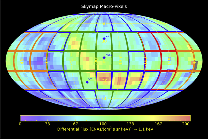
Figure 2. Selected 56 macropixels overlaid on a representative IBEX-Hi ENA map for reference. The color-coding of the pixel boundaries indicates the degree of confidence in the derived HP distances, as described in Section 3.5. Green indicates category 1 pixels, where the best-fit time correlation coefficient is greater than 0.75; blue indicates category 2 pixels (correlation coefficient between 0.25 and 0.75); orange indicates category 3 pixels (tailward pixels); and red indicates category 4 pixels (see text). The upwind direction ("nose") and the locations in the sky of Voyagers 1 and 2 ("V1" and "V2") are also called out.
Download figure:
Standard image High-resolution imageFor the top four energies (1.1–4.29 keV), the statistical uncertainties in the macropixels are in the 1%–4% range (1σ), except at the poles, where the uncertainties are ∼0.2%, because the exposure times are nearly continuous. At 0.71 keV, the mean statistical uncertainty is somewhat higher, at 6%, due to the lower sensitivity of the IBEX-Hi instrument at this energy. For a few macropixels where heliospheric viewing is limited by foreground contamination (e.g., the Earth's magnetosphere and magnetosheath), the statistical variation is considerably larger, as discussed in Section 3.5. Note that the macropixel averaging does not remove systematic variations that can impact the time correlation. There are still variations in the data from imperfect subtraction of background and limitations of the accuracy of the CG correction method as noted by McComas et al. (2018a). The cases where statistical and systematic noise do have an impact on the analysis will be noted.
3. Sounding the Distance to the Heliopause
The principle underlying the sounding method is that dynamic pressure variations in the outbound SW will induce corresponding variations in the HS thermal pressure, which, in turn, will affect the intensity of the ENA signal observed by IBEX. If one can uniquely trace time-varying features in the ENA signal back to time-varying features in the 1 au SW dynamic pressure observed years before, and if one knows the propagation speed of all of the relevant particle components, then one can determine the average distance to the ENA source region. We say "average" because, due to the thickness of the source region, ENAs will be formed at a range of distances along the LOS from IBEX. We take "average" to mean the median distance of ENA formation along the LOS. To apply the sounding method outside the ecliptic, we assume that measurements of the SW dynamic pressure in the ecliptic are valid at other heliolatitudes. Indeed, the SW dynamic pressure has been shown to be invariant with heliolatitude based on Ulysses observations (McComas et al. 2008), at least on the timescales of relevance here (∼a few months).
The sounding method was applied to IBEX data by Reisenfeld et al. (2012, 2016) by correlating the observed SW dynamic pressure at 1 au with the polar ENA flux observed years later to determine the distance to the HP at the ecliptic poles. Zirnstein et al. (2018) used a heliosphere simulation to test the validity of the method to find the distance to the HP in all directions in their simulated heliosphere. A pressure disturbance is "propagated" through their model, and a simulated ENA flux is calculated. Figure 3 shows the results of the simulation, reproduced from Zirnstein et al. (2018). Employing the method described below, the colored curves in the figure show the estimated location of the simulated HP in the equatorial plane based on simulated 1.11 (orange) and 4.29 (red) keV ENAs. We see that in the upwind hemisphere and slightly tailward, the HP position is accurately determined for both energies to within ∼10 au. For most of the downwind hemisphere, the boundary based on the 4.3 keV ENA is underestimated because of the loss of energetic HS protons to charge exchange before they can propagate to the HP. In Section 4, we will use this method to determine the boundaries of the actual HP in all directions utilizing IBEX observations, with the understanding that for the downwind hemisphere, the results are interpreted as lower limits on the HP distance, as the actual downwind HP could be much further away. Here we summarize the sounding method, highlighting key elements.
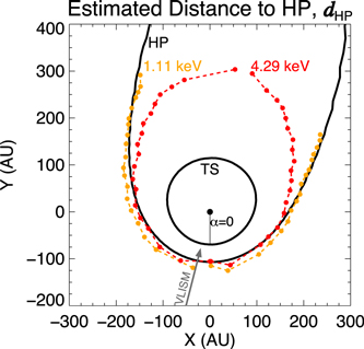
Figure 3. Estimation of the distance to the HP in the Zirnstein et al. (2018) simulation using the sounding method. The location of the simulated HP is shown in black, and the estimated distances to the HP based on applying the sounding method to the simulated flux of ENAs at 1.11 (corresponding to IBEX-Hi ESA 2) and 4.29 (ESA 6) keV are shown in orange and red, respectively.
Download figure:
Standard image High-resolution image3.1. The Trace-back Time
Given an SW disturbance propagating outward at the SW speed vSW at a particular longitude b and latitude λ, the delay time it takes for the effect of that disturbance to be observed in the return ENA signal is estimated by Equation (3) of Zirnstein et al. (2018),
where  is the average trace-back time for ENAs originating in the HS and detected in the ith energy passband of IBEX-Hi, dTS and lHS are the (unknown) TS distance and HS thickness, vms is the average magnetosonic speed in the HS, and vENA(E) is the speed of an ENA observed by IBEX at a solar rest-frame energy E.
The first term on the right-hand side is the time it takes for an SW parcel to travel from the Sun to the TS. The second term is the time it takes a pressure pulse generated at the TS traveling at the magnetosonic speed to propagate to the HP and halfway back. This takes into account the finding of McComas et al. (2018a) and Zirnstein et al. (2018) that only after a pressure pulse rebounds from the HP and propagates back to the TS does the plasma pressure fully adjust to a change in the SW dynamic pressure. The reason we use the time it takes for the pulse to only propagate halfway rather than all the way back to the TS is because we are calculating the average trace-back time for ENAs formed between the HP and the TS, and we assume that the midpoint of the HS is the average formation point for ENAs. The last term represents the time it takes ENAs formed at the midpoint to travel back to IBEX.
In this work, the period of observation is a full solar cycle; so, to arrive at realistic values for ttb, we need to account for changes in the SW speed as a function of latitude over the solar cycle; this is especially important for high latitudes, which have much higher speeds on account of the large circumpolar coronal holes around solar minimum, compared to slower and more variable speeds around solar maximum (e.g., McComas et al. 1998). We therefore calculate time-dependent SW speeds using the method of Sokół et al. (2015, 2020) in which SW speeds over time and versus latitude are derived from interplanetary scintillation (IPS) observations (Tokumaru et al. 2012). Details of the derivation of the SW speed from multistation IPS measurements, which are used in the method by Sokół et al. (2015, 2020), are given in Tokumaru et al. (2010). Note that, as in Reisenfeld et al. (2016), we reduce the outgoing SW speed by 10% from these observed values to account for the deceleration of the SW due to mass loading by pickup ions. For vms, we use a value of 314 km s−1, the HS magnetosonic speed derived from Voyager observations by Rankin et al. (2019).
3.2. The LOS-integrated Pressure of the HS
The action of the SW dynamic pressure can be related to the ENA flux observed by IBEX-Hi via the plasma pressure integrated over the LOS through the HS (see Schwadon et al. 2011):
The limits of integration span the energy range of IBEX-Hi CG-corrected observations of the ENA flux jENA(E), where E is the ENA energy in the Sun's rest frame, and v is the corresponding velocity. Thus, Equation (2) does not account for the total HS pressure, as there are significant contributions from outside the IBEX-Hi energy range. However, we expect this energy range (0.5–6 keV) to be the range most sensitive to variability in the outgoing SW and its associated pickup ions. Since we are interested in tracking variations and less interested in the absolute pressure, the fact that we are not measuring the total HS pressure is not of concern. The other quantities on the right-hand side of Equation (2) are m, the proton mass; nH, the interstellar neutral hydrogen density, taken to be 0.127 cm−3 (Swaczyna et al. 2020); and σ (E), the charge-exchange cross section (Lindsay & Stebbings 2005).
The quantity PS denotes the "stationary" pressure, or the internal pressure of the HS plasma if it were at rest in the Sun's rest frame. The distance L is the thickness of the primary ENA-forming region, interpreted here as the thickness of the HS. The product PS •L is referred to as the "LOS-integrated pressure," and it is determined entirely by observations. As pointed out by Schwadron et al. (2011), the nonstationary component of the LOS-integrated pressure scales more or less linearly with the stationary component; thus, for the purpose of correlating changes in the HS with the 1 au SW dynamic pressure, it is sufficient to work with PS •L.
In practice, since ENAs are measured in discrete energy passbands, the integral in Equation (2) must be calculated in a piecewise manner. We assume that jENA(Ei ) is a measurement of the flux precisely at the central energy Ei of the ith passband, and that the flux between adjacent central energies follows a power law with spectral index γi . Then, Equation (2) can be evaluated by the sum of a set of LOS-integrated partial pressures:
Note that ENAs detected in the different passbands of IBEX-Hi have different trace-back times. This means that to carry out the time correlation, the energy integral in Equation (2) must be performed by summing over the five partial pressures given by Equation (3), each with a different time offset.
3.3. Carrying Out the Time Correlation
In order to determine the distance to the ENA-forming region, we time-correlate HS plasma pressures calculated using Equations (1)–(3) with 1 au SW dynamic pressure observations. We will now walk through the steps in this procedure by reference to Figure 4, which shows the sounding method applied to a macropixel centered at the ecliptic longitude/latitude of (−75°, 30°). Figure 4 (top panel) shows partial and total LOS-integrated plasma pressures in the HS versus the trace-back date, that is, the IBEX observation date minus the trace-back time: tIBEX − ttb. The total pressure given by Equation (3) (black curve) is calculated from the partial pressures (colored curves) for the date range when the trace-back dates for all five IBEX-Hi energy passbands overlap. The total pressure curve is scaled arbitrarily to keep it on the same plot range as the partial pressures.
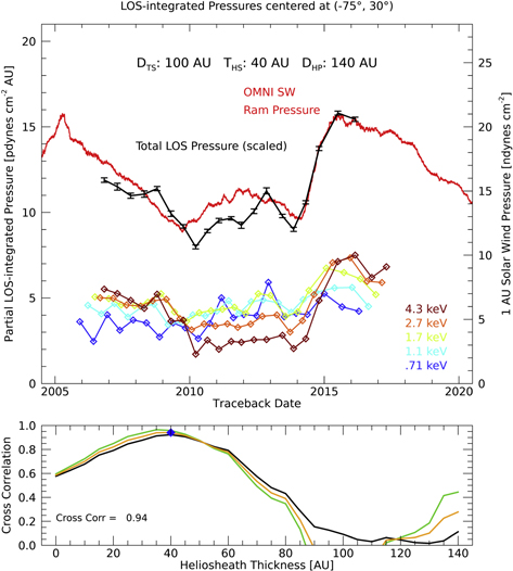
Figure 4. (Top) Partial and total LOS-integrated plasma pressure in the HS vs. trace-back time (Equation (1)) for the macropixel centered at (−75°, 30°). This is for the case of a TS distance of 100 au and a best-fit HS thickness of 35 au, leading to an HP distance of 135 au. The partial LOS-integrated pressures (colored curves) are derived using Equation (3), and the total LOS-integrated pressure (black curve) is calculated from the partial pressures (Equation (2)) for the range where the trace-back times for all five ESA steps overlap. Also shown is the 1 au SW dynamic pressure calculated from the OMNI data set (red line) plotted at the actual time of observation. Statistical uncertainty error bars (1σ) are shown on the total pressure points. For clarity, they are not shown on the partial pressures. (Bottom) The choice of trace-back times shown in the top panel is based on varying the HS thickness between zero and 140 au. For each choice of HS thickness, the cross-correlation coefficient is calculated for the entire time series of flux measurements (black line) and only the last 5 yr (green line) in order to emphasize the correlation with the rapid increase in pressure observed at 1 au in 2014. The orange line is the arithmetic mean of the two. The blue diamond indicates the best correlation coefficient and therefore the best-fit HS thickness.
Download figure:
Standard image High-resolution imageAlso shown in Figure 4 (top panel) is the 1 au SW dynamic pressure calculated from the OMNI-2 SW archive (red line; King & Papitashvili 2005), plotted at the actual times of observation. This curve is smoothed by a 1 yr running average to remove annual oscillations due to the ±7° yearly excursion of the Earth in heliographic latitude. The smoothing is also warranted because the propagation time of a pressure pulse through the HS to the HP and back is of order a year; thus, the ENA flux collected along the LOS will be effectively smoothed on this timescale.
The "best" trace-back time is dictated by evaluating the correlation between the total HS plasma pressure and the 1 au SW dynamic pressure for a range of HP distances. Examining Equation (1), we see that the sounding method does not uniquely determine both dTS and lHS; thus, we must use an alternate means of fixing one of these. Since dTS is perhaps better constrained by other methods, we fix dTS and vary lHS in the cross-correlation calculation (Figure 4, bottom panel). For the example presented here, we set dTS = 100 au (the rationale for this will be discussed in Section 3.4) and then vary lHS between zero and 140 au in 5 au increments. For each value of lHS, the cross-correlation coefficient is evaluated. Taking the peak cross-correlation coefficient, we find that a best-fit value for lHS is 35 au (blue diamond in bottom panel), leading to an HP distance of 135 au.
The correlation in this example is of excellent quality, with a high maximum correlation coefficient of 0.94. The results are not always this unambiguous because there is sometimes considerable systematic noise in the ENA data, as discussed in Section 2.3, which can complicate the correlation analysis. Fortunately, the Sun has given us some help. Inspecting the correlation between the total LOS pressure and the SW dynamic pressure, the dominant feature driving the correlation is the rapid rise in the SW dynamic pressure that occurs in 2014. This pressure enhancement later appears in the IBEX-Hi ENA observations starting in late 2016. It first shows up at 4.3 keV, appearing as a strong enhancement ∼30° south of the interstellar upwind direction, and then expands outward in each successive sky map (McComas et al. 2018b, 2019a). The enhancement appears at lower energies later than at the top energies, which is a consequence of the longer travel times for lower-energy ENAs from the HS to IBEX. By the end of 2019, the ENA enhancement has spread to encompass roughly two-thirds of the sky at 4.3 keV (McComas et al. 2020).
In the regions of the sky where the ENA enhancement associated with the 2014 dynamic pressure enhancement is present, it turns out that the cross-correlation results are much more stable pixel-to-pixel if the ENA enhancement is given more weight. This is done in practice by carrying out two correlations, one for the full time series (black line in Figure 4, bottom panel) and one for only the last 5 yr of the time series (green line), where the pressure enhancement dominates. We then take the arithmetic mean of the correlation coefficients (orange line) and assign the best trace-back time to the maximum of the mean correlation. In this manner, we give additional weight to the pressure enhancement but still use information from the full time series to set the HP distance. Note that in this case, it does not matter which correlation is used, since both correlation methods peak at the same choice of HS thickness. As we will see in Section 3.5, using the weighted cross-correlation makes a difference. In regions of the sky that the pressure enhancement has not reached, we simply use the full time series correlation.
We note that the boundaries of the TS and HP change with time to maintain the pressure balance between the SW and interstellar medium (ISM) total pressures. Since the SW pressure is dominated by the dynamic pressure of the outflowing supersonic wind, which evolves throughout the solar cycle, this can cause the boundaries to move. The question therefore arises as to the validity of carrying out a time correlation across 11 yr to determine the distance to the HP if the HP is in constant motion. Time-dependent studies that use realistic inputs for the variability of the SW over the solar cycle predict that the TS distance varies by perhaps ∼±10 au and the HP by even less, ∼±5 au (Izmodenov et al. 2005; Washimi et al. 2011; Izmodenov & Alexashov 2020). As we discuss in Section 3.5, we estimate the uncertainty in the distance to the HP based on the sounding method to be at best ±10 au; thus, the expected temporal motion of the HP is well within the method's uncertainties. Furthermore, as we shall see in Section 4, the derived distance to the HP is fairly insensitive to the choice of TS model (see next section), even though there is considerable variation in TS distances between the models, a variation that is larger than the ±10 au variation of the TS distance over the solar cycle. Therefore, we do not expect the time variation of the TS and HP distances to significantly affect our results.
3.4. Choosing the TS Distance
As mentioned in the previous section, the pressure correlation technique does not uniquely determine both the TS distance and the HS thickness. We therefore have assumed different shapes for the TS and then evaluated the distance to the HP using TS distances derived from these shapes. Another reason for using different TS models is that this will tell us how sensitive the resulting HP shapes are to the choice of TS shape. We carry out the procedure with three models.
- 1.A uniform Sun-centered 100 au radius TS model. This is chosen to demonstrate that the resulting HP distance variations are driven not by any inherent asymmetry in the TS model but rather by the ENA data themselves.
- 2.The spherical TS shape derived by the McComas et al. (2019b) analysis of ACRs measured by the two Voyager spacecraft as they traversed the IHS (the Voyager TS model). As described in the Introduction, this analysis provides a best-fit spherical TS with a radius of 117 au and a center offset from the Sun. Although the true TS shape is not likely to be purely spherical, it does represent the simplest shape that can be fit to four points: the two Voyager TS crossing points and the derived locations of the TS boundary in the tail. This TS model is used because it represents the most data-driven approach to finding the shape of the HP that can be used at this time and also yields an asymmetric TS shape qualitatively similar to that expected from previous IBEX data analyses (e.g., Schwadron et al. 2014; Reisenfeld et al. 2016; Zirnstein et al. 2017a; McComas et al. 2020).
- 3.A TS shape derived from the MHD-plasma/kinetic-neutral model of Zirnstein and Heerikhuisen (the Z-H TS model). The Z-H model solves ideal MHD equations for the SW and interstellar plasmas, treated as a single fluid, and Boltzmann's equation for neutral H atoms, treated kinetically (e.g., Pogorelov et al. 2008; Heerikhuisen & Pogorelov 2010). In their model, SW data from the OMNI database are used to represent SW conditions up to 37° from the solar equator, and Ulysses measurements are used for SW conditions for latitudes above 37°, thus approximately reproducing solar-minimum conditions in solar cycle 23 and yielding a nearly latitude-independent SW dynamic pressure. The local ISM boundary conditions (i.e., ISMF, plasma and neutral density, flow velocity, temperature) are derived from a combination of multi-spacecraft measurements (for more details, see Zirnstein et al. 2021). The rationale for the use of such a model is that this gives us a TS shape driven by detailed heliospheric physics, including kappa-distributed protons in the HS, the draping of the ISMF around the HP consistent with IBEX ribbon measurements, and reproduction of the average TS distances observed by Voyagers 1 and 2 (∼89 au).
3.5. Correlation Behavior across the Sky
The time correlation is carried out for each of the 56 macropixels shown in Figure 2 and repeated for each of the three TS models using the method described in Section 3.3. The best-fit HP distance is taken as that which gives the maximum cross-correlation coefficient. There is a great deal of variation in the appearance of the ENA time series, depending on the region of the sky, and a corresponding variety in the quality of the correlations between the ENA and SW time series. To assess the quality of the correlations, we categorize the correlation behavior of the different sky pixels into four categories. Here we describe each category and look at representative examples. These are all taken from the runs with the 100 au TS model, but what we describe applies generally, as the correlations behave nearly the same for all of our TS models.
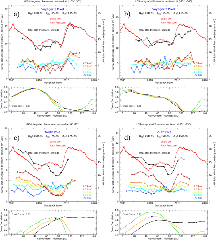
Category 1. The first group is the largest category and consists of 21 pixels (38% of the total) having correlations that look very similar to the (−75°, 30°) pixel shown in Figure 4. As shown by the color-coding in Figure 2, these pixels are located in the upwind hemisphere, spanning from the equator to high latitudes (but not the polar pixels). All but two of these pixels are within 75° longitude of the upwind direction. The ENA time series is characterized by a well-defined pressure enhancement, and it closely follows the SW time series across the entire time span. For all of these, the best-fit correlation coefficient is greater than 0.75. Contained in this category are the V1 and V2 pixels, centered at (−105°, 30°) and (−75°, −30°), respectively (Figures 5(a) and (b)). Also in this category is the nose pixel (−105°, 0°). Because of the tightly constrained correlations of the category 1 pixels, a significant drop in the quality of the correlation is readily visible by making quite small time shifts. We therefore set the uncertainty in the best-fit time correlation at the resolution of the ENA time series, or ±3 months (half the time between sky maps). This corresponds to changing the assumed HP distance by ±10 au. We therefore set the uncertainty in the HP distance for category 1 pixels at ±10 au.
Download figure:
Standard image High-resolution image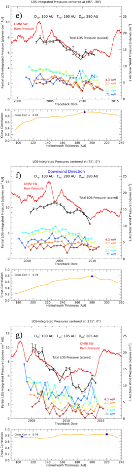
Figure 5. Panels (a) and (b) are examples of category 1 pixels (see text), and panels (c) and (d) are examples of category 2 pixels. See caption to Figure 4 for description of plots. Panels (e) and (f) are examples of category 3 pixels (see text), and panel (g) is an example of a category 4 pixel. See caption to Figure 4 for description of plots.
Download figure:
Standard image High-resolution imageThe fact that the ENA time series consistently track the SW dynamic pressure even up to high latitudes provides strong supporting evidence for the idea that the SW dynamic pressure is a latitude invariant. This is an important assumption for this study, because without it, the ability to apply the sounding method would be limited to only the ecliptic. This assumption also factors into the reconstruction of the SW density profiles as a function of heliolatitude from the SW speeds derived from IPS observation data (Sokół et al. 2015, 2020). Our work indirectly relies on these SW density profiles, as they are used to calculate ENA survival probabilities applied to the IBEX data (Bzowski 2008; McComas et al. 2017, 2020, Sokół et al. 2020).
Category 2. The next category consists of pixels where the correlation is anchored by a well-defined pressure enhancement as in category 1, but the ENA time series does not necessarily cleanly track the SW time series. This category is almost as large as category 1, consisting of 20 pixels (35%). It includes the high-latitude pixels not in category 1, including the polar pixels (see Figure 2). At equatorial/low latitudes, it includes pixels on the flanks of the heliosphere as far as 105° from the upwind direction. Correlation coefficients range from as low as 0.23 up to 0.79. Even though the peak correlations are not as high as for the category 1 pixels, the pressure enhancement still puts a reasonably tight constraint on the HP distance. To quantify this, we look at how much the HP distance must change to reduce the correlation coefficient by 0.1. This varies somewhat from pixel to pixel but is in the range of ±10–20 au; thus, we put the typical uncertainty on category 2 pixels at ±15 au.
Because of their significance in previous work (Reisenfeld et al. 2012, 2016), correlations for the north and south polar pixels are shown in Figures 5(c) and (d), respectively. The statistical uncertainties for these two pixels, at 0.2%, are exceptionally low because the poles are observed continuously throughout the IBEX mission. Note now that the different correlation cases (green and black lines) look quite different from each other, in contrast to Figures 5(a) and (b). The mean of the coefficients (orange line) provides a more stable determination of the HS thickness. Although the correlations with the SW time series are not as tight as they are for category 1 pixels, they are still quite good, with coefficients of 0.65 for the north pole and 0.73 for the south.
The pixels that fall into category 2 are consistently further from the nose than the category 1 pixels. A possible explanation for the drop in the quality of the correlation for category 2 pixels is that because they are more distant from the upwind direction, the HS plasma at these locations is not only responding to pressure signatures radially transmitted across the TS but also to pressure structures convecting tailward within the HS; thus, pressure changes are due to an admixture of these two drivers. Fortunately, the 2014 pressure enhancement is large enough to dominate the internal processing, giving us a strong feature to correlate on.
Category 3. This category consists of pixels in which the 2014 pressure enhancement has yet to show up in the ENA time series. Not surprisingly, this consists exclusively of downwind pixels, numbering 10 in total (18%). They are all equatorial or low latitude and at least 105° in longitude from the upwind direction. The best-fit correlation coefficients are high; all but two are above 0.80, with the lowest at 0.68 and the highest at 0.93. This is in part due to the fact that there is not a lot of structure to correlate on, as the ENA time series for these pixels tends to have a flat downward slope that matches the general trend in the SW time series between 2003 and 2010. That is, the cross-correlation coefficient between two similarly sloped straight lines is intrinsically high.
Figure 5(e) shows the correlation for a typical pixel, centered at (45°, −30°) (located on the downwind, starboard side), having an "HP distance" of 290 au. This pixel has a peak correlation coefficient of 0.930, but we can see that the correlation is good for a very broad range of HS thicknesses for the reason above; thus, it is not clear how well constrained the distance is. We place "HP distance" in quotes because we now have to modify our interpretation of this distance when applying it to the downwind portion of the heliosphere. If the HP truly does truncate the heliosphere approximately at this distance in the tail, then this interpretation is fine. However, as we noted at the beginning of Section 3, due to the finite lifetime of the HS plasma parent to the observed ENAs, this must really be interpreted as a lower limit on the distance to the HP. In principle, the heliotail could extend hundreds of au downwind and we would never know it. Strictly speaking, the distance we have derived is simply the distance to the far edge of the ENA-forming region for ENAs in the IBEX-Hi energy range.
Figure 5(f) shows the directly downwind (antinose) macropixel at (75°, 0°), which has a peak cross-correlation coefficient of 0.77 occurring at a distance of 380 au. This value probably has a large uncertainty, but that said, given the overall shape of the ENA time series, its phasing with the SW time series strongly suggests that the ENA source must be of order 350+ au downwind. These broad correlation ranges are typical for category 3 pixels, and we place the uncertainty on the distance to the edge of the ENA formation region at ±30 au.
Category 4. The final category consists of a small number of macropixels where the ENA time series is particularly noisy, and for this reason, the cross-correlation analysis has a very high uncertainty. For these pixels, the cross-correlation is flat across a wide range of HS thickness values, leaving the choice of HS thickness ambiguous. Five pixels (9%) fall in this category, located in a part of the sky where IBEX's view of the heliosphere is partially obscured by the Earth's magnetosphere and magnetosheath; thus, there is limited usable data. This band, between ecliptic longitudes 120° and 150° on the starboard flank and 0° and 30° on the port flank, contains large amounts of statistical variability, which is further amplified by the CG correction. As a result, much of the structure in the ENA time series is noise, leading to false correlations. In these cases, we are forced to manually adjust the choice of HP distance based on patterns in the ENA time series from adjacent longitudes or the arrival of the pressure enhancement in the last few high-energy points. Figure 5(g), for the (135°, 0°) pixel, clearly shows the high level of statistical fluctuation in the ENA partial pressures, as well as a very flat correlation coefficient curve across a large range of HS thicknesses. The blue circle in the lower panel shows the calculated peak correlation at lHS = 195 au, and the blue diamond shows the manually selected HS distance, lHS = 100 au.
A list of the distances to the TS and HP for each of the 56 pixels and three different TS models, as well as the correlation coefficients for the given choice of HS thickness, is available in the online-only material as an Excel spreadsheet. The next section describes the shape of the heliosphere based on these distance determinations.
4. The Shape of the Heliosphere
Figures 6–8 show orthogonal views of the derived shape of the heliosphere for each of the three TS models: the uniform 100 au TS (Figure 6), the spherical fit to the TS distances derived from the analysis of Voyager data (Figure 7), and the TS distances from the Z-H MHD model (Figure 8). (Interactive versions of these renderings are available as online-only material.) A modified ecliptic coordinate system is used, where the z-axis is directed along the ecliptic poles, the y-axis is aligned with the longitude of the heliospheric nose (−105° longitude in J2000 ecliptic), and the x-axis completes the right-hand triad. The red cone shown in the images indicates the direction of the ISMF far (∼1000 au) from the Sun, determined by Zirnstein et al. (2016) to be (227 28, 3462) in ecliptic longitude and latitude, based on their analysis of the IBEX ribbon. A complementary representation of the heliosphere boundaries is given in Figure 9, which represents distances in the form of color maps for the TS distance, HS thickness, and HP distance for each of the TS models. These are presented as standard Mollweide projections centered on the upwind direction from the vantage of the Sun.

Figure 6. Orthogonal views of the 3D shape of the heliosphere using the 100 au TS model. The HP is represented in cyan, the embedded TS is green, and the Sun is represented by the yellow dot at the center of the coordinate axes. Axis units are in astronomical units. The positive y-axis points in the upwind direction, and the positive z-axis points toward the north ecliptic pole. The red cone represents the direction of the far interstellar magnetic field at ∼1000 au as determined by Zirnstein et al. (2016). See text for discussion. The online interactive image can be rotated and zoomed using standard gestures, depending on the operating system (e.g., slide two fingers up or down or use the mouse wheel to zoom in and out, click and drag to rotate, etc.), or using the menu at the top of the figure (much slower and not recommended). Note that the interactive graphic appears in full with the current versions of the Chrome, Firefox, and Edge browsers.(An interactive version of this figure is available.)
Start interactionDownload figure:
Standard image High-resolution image Figure data file
Figure 7. Orthogonal views of the 3D shape of the heliosphere using the Voyager-derived TS model. See Figure 6 for further details.(An interactive version of this figure is available.)
Start interactionDownload figure:
Standard image High-resolution image Figure data file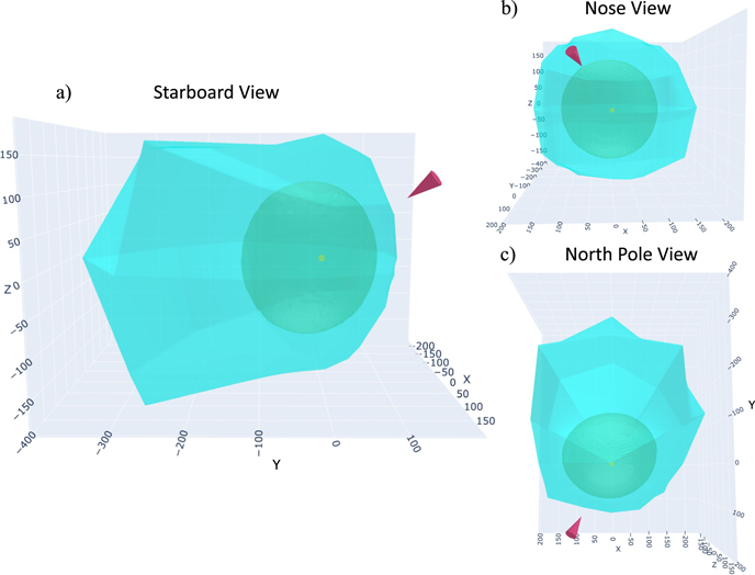
Figure 8. Orthogonal views of the 3D shape of the heliosphere using the Z-H TS model. See Figure 6 for further details.(An interactive version of this figure is available.)
Start interactionDownload figure:
Standard image High-resolution image Figure data file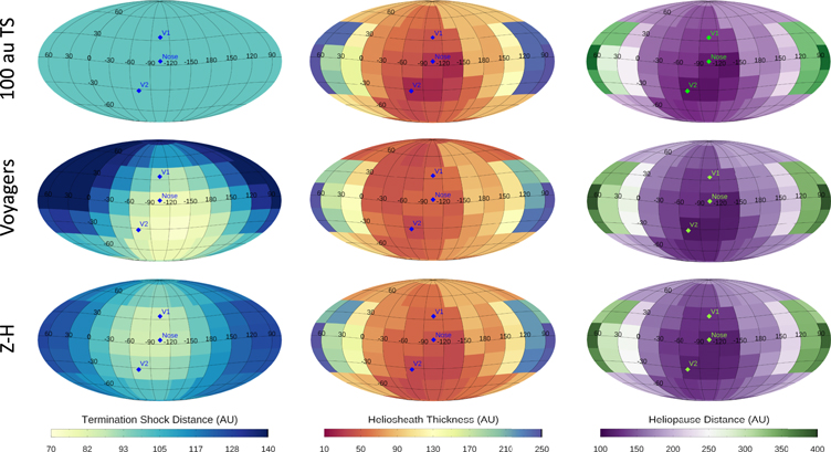
Figure 9. Heliospheric distances represented as color maps for (left to right) the TS distance, HS thickness, and HP distance for each of the three TS models. These are Mollweide projections centered on the upwind direction, as viewed from the Sun.
Download figure:
Standard image High-resolution image5. The Heliopause
It is clear from Figures 6–9 that the shape of the HP is nearly independent of the choice of TS model, demonstrating the stability with which the sounding technique determines the HP distance. We see that the shape is determined primarily from the interaction of the heliosphere with the ISM flow, as the HP can be seen to clearly drape around the TS away from the upwind direction. The ISMF also affects the shape of the HP, but in a secondary manner. We observe from Figure 9 that the region of minimum radial distance to the HP is 110–120 au, depending on the TS model. This region is not centered on the nose pixel but rather is located south of the nose and toward the starboard flank. (Note that the coarse resolution of the macropixel map does not allow for localization of the minimum HP distance to better than ∼20° or so.) This is qualitatively consistent with the observations by McComas & Schwadron (2014) that the HS pressure maximum is offset ∼20° south of the nose and slightly toward the starboard flank, owing to the action of the magnetic force from the tilted ISMF. Another indication that the ISMF influences the shape of the HP is that, as can be seen in Figures 6–8, the downwind side of the HP appears to be deflected slightly to the port side and southward, away from the direction of the ISMF. This deflection may be an indication of squeezing of the heliotail by the ISMF, which would shift the HP in the port-south and starboard-north directions along the B–V plane. However, this shift appears to be only a minor effect considering the uncertainties of our results.
Figures 6–8 show the HP boundary extending to about 350 ± 50 au in the downwind direction. As discussed in Section 3, the application of the sounding technique in the tail is limited to about this distance by the loss of ions in the IBEX-Hi energy range via charge exchange. Therefore, all we can say is that the HS extends to at least ∼350–400 au downwind from the Sun, but we cannot rule out the possibility that it extends much further. This means that our analysis is unable to distinguish between heliosphere models that predict a long comet-like tail extending downwind thousands of au (e.g., Izmodenov & Alexashov 2015; Pogorelov et al. 2015, 2017) and a more compact heliosphere with an HP located only 300–400 au from the Sun (e.g., Opher et al. 2015, 2020). Note that this distance is consistent with the estimated thickness of the downwind HS of 220 ± 110 au by Galli et al. (2016) after adding in the TS distance of ∼100–150 au (depending on TS model), as well as the estimated distance to the ENA source in the heliotail of ≳290–490 au from Zirnstein et al. (2020). However, these results indicate that the derived distance of the HP toward the tail of ∼200 au by Dialynas et al. (2017) using Cassini/INCA data is not correct.
At high latitudes, the HP extends to about 175 au in the north and 150 au in the south. Note that this is independent of the choice of TS model, to within 5 au or so. We note that the north pole HP distance is 15 au further than derived by Reisenfeld et al. (2019) but at the limit of the estimated ±15 au error, and the south pole HP distance is in agreement with Reisenfeld et al. (2019). These distances are somewhat shorter than predicted by heliosphere models, which predict distances to the HP at the poles ranging from ∼200 (e.g., Zirnstein et al. 2017b) to ∼300 (e.g., Opher et al. 2020) au. At these distances, we do not expect the extinction effect to be significant; thus, the derived distances for the high-latitude ( ) pixels should be accurate. The views from the flank side in Figures 6–8 show that the high-latitude HP boundary has more of a "bullet" shape, consistent with the heliosphere model of Pogorelov et al. (2013) and Izmodenov & Alexashov (2020), than the "croissant" shape described by Opher et al. (2015, 2020), which predicts an HS that extends much further above the poles than our observations show.
5.1. Choice of TS Model
Although the shape of the HP is nearly independent of the choice of TS model, this does not mean that there are no important model-dependent differences to the heliosphere structure, particularly with regard to the thickness of the HS.
We first consider the 100 au TS model. As stated in Section 3.4, this model was chosen to demonstrate that asymmetries in the derived HP were not artifacts of the choice of TS model. In a sense, the 100 au TS acts as a "control" for the other models. Since it is not a particularly realistic TS model, we should not place much weight on conclusions drawn from it about the shape of the HS. For instance, in the region south of the nose where the minimum HP distance is 115 au, the HS appears to be about 15 au thick, which would seem unreasonably thin in light of pretty much any theoretical model of the HS. We know that since this region includes the pixel containing the Voyager 2 TS crossing, the TS distance in this region is more like 80–90 au, so the 100 au TS leads to an underestimate of the HP thickness there.
By design, the Voyager-based TS model (McComas et al. 2019b) accurately depicts the TS distance at the Voyager TS crossings, which means it likely represents the TS distance fairly well in regions near the nose. However, the four points defining this spherical model are all within 30° of the ecliptic, so the TS is not nearly as well constrained at high latitudes. Indeed, at high northern latitudes, the model predicts a TS distance of ∼150 au, which is likely an overestimate, as this leads to an HS thickness of 30–40 au, which for this model is as thin as it is around the nose, where we expect the HS to be at its thinnest owing to the nose being where the ISM flow and field exert maximum pressure. This result is also inconsistent with numerical models (e.g., Pogorelov et al. 2013; Izmodenov & Alexashov 2020). To be clear, McComas et al. (2019a, 2019b) did not claim that the TS is strictly spherical; rather, they fit an offset spherical shape on purely empirical grounds, as this is the most complex shape constrained by a four-point fit, which is the number of observed points.
Turning to the Z-H TS model, the shape of the TS is largely independent of latitude because the distance to the TS is determined by SW dynamic pressure, which is approximately latitude-independent, even though the SW speed varies significantly with latitude. Even during solar maximum, when the fast SW disappears, the Z-H TS model predicts a similar TS shape to solar minimum, so long as the SW dynamic pressure does not significantly change over time. Moreover, this model is constrained to reproduce the averaged TS crossing distances from Voyagers 1 and 2 (∼89 au), but it would need to incorporate time dependence to explain the observed ∼10 au asymmetry. This model provides a representation of the TS shape based on our best understanding of heliospheric physics. (Note that between the various heliospheric modeling research groups, although there is a wide range of predicted shapes for the HP, there is far less variation in the modeled TS itself.) Figures 8 and 9 show that the resulting HS is thinnest near the region of maximum compression by the LISMF and thicker over the north pole than the south and flares symmetrically about the port and starboard flanks of the TS.
5.2. The Voyager 1 and 2 Pixels
Our global depiction of the heliosphere intersects with direct observation in two regions of the sky, in the pixels containing the Voyager 1 and 2 TS and HP crossings. This provides a means of validating the sounding method, at least for the upwind hemisphere. Table 1 gives the distances to these boundaries and the thickness of the HS for the three versions of the TS model and compares them to the distances determined from the Voyager 1 and 2 crossing distances. Note that the values for the Voyager model TS distances do not exactly match the actual Voyager distances because these pixels are averages over a 30° × 30° area of the sky.
Table 1. Comparison between the Sounding Method and Observation for Voyager 1 and 2 Distances
| Pixel Location | Model | TS Distance (au) | HS Thickness (au) | HS Thickness Difference from Voyager (au) | HP Distance (au) | HP Distance Difference from Voyager (au) | |
|---|---|---|---|---|---|---|---|
| Voyager 1 | Actual | 94 | 28 | ⋯ | 122 | ⋯ | |
| 100 au TS | 100 | 35 | 7 | 135 | 13 | ||
| Voyager TS | 91 | 45 | 17 | 136 | 14 | ||
| Z-H TS | 86 | 45 | 17 | 131 | 9 | ||
| Voyager 2 | Actual | 84 | 35 | ⋯ | 119 | ⋯ | |
| 100 au TS | 100 | 15 | −20 | 115 | −4 | ||
| Voyager TS | 82 | 30 | −5 | 112 | −7 | ||
| Z-H TS | 95 | 30 | −5 | 120 | 1 |
Download table as: ASCIITypeset image
The last column shows that the sounding method accurately determines the distance to the HP for the V2 pixel to well within the uncertainty of the method (±10 au). The HS thickness determined using the Voyager and Z-H TS models of 30 au is also quite close to the observed HS thickness of 35 au. It is no surprise that the 100 au model underestimates the HS thickness, since the TS distance is an overestimate. For the V1 pixel, the HP distances are consistently higher than the observed Voyager 1 HP crossing distance but are still at or near the uncertainty of the method. One must also keep in mind that the Voyager crossings only indicate the boundary locations at one point in time, and that the TS and HP boundaries have quite likely moved relative to one another by order of 5–10 au between their respective crossings by Voyager.
On the whole, the comparison to the Voyager distances validates the sounding method for determining accurate distances to the HP. Coupled with what we expect are realistic models of the TS, it is possible to determine a reasonably accurate measure of the thickness of the HS as well.
6. Summary
We have used a full solar cycle of IBEX-Hi ENA flux data, combined with 1 au SW observations, to determine the distance to the HP. This is done by correlating the time variation in the ENA-derived HS plasma pressure determined from 22 consecutive 6 month ENA maps with earlier measurements of the 1 au SW dynamic pressure. We apply this sounding method to each of 56 macropixels spanning the entire sky. To ensure we are using only ENAs of HS origin to calculate the plasma pressure, we apply a new technique to remove IBEX ribbon flux from each of the 22 ENA maps, leaving only the GDF.
We must also assume that the SW dynamic pressure is a latitude invariant, as implied by Ulysses observations (McComas et al. 2008). We find that when the sounding method is applied to high-latitude pixels, there is a very good time correlation between the HS plasma pressure and the SW dynamic pressure. This is important additional evidence for the latitude invariance of the dynamic pressure.
The time shift giving the best correlation is used to derive a distance to the HP in the direction of each macropixel. Because the HP distance also depends on the TS distance, we make use of various TS models. We find that to within the estimated uncertainties of the sounding method, the derived HP distances do not depend strongly on the choice of TS model.
The quality of the time correlation varies considerably across the sky, so we divide the macropixels into four categories. Category 1 pixels are all located in the upwind direction and have well-constrained correlations strongly tied to the pressure enhancement. We have assigned their derived HP distances an uncertainty of ±10 au. Category 2 pixels are located along the flanks, at the poles, and at high latitudes away from the upwind direction. The time correlations for these pixels are still significantly anchored to the pressure enhancement but not as tightly. The uncertainties in their HP distances are a little broader, ±15 au. Category 3 pixels are all in the tail, and because the pressure enhancement has yet to reach the tail, the correlations are much less well constrained, and the assigned uncertainty is ±30 au. Finally, category 4 pixels have correlations marred by large uncertainties in the ENA flux and required manual time shifting based on either (a) comparison to adjacent, less noisy pixels or (b) the appearance of the pressure enhancement at the higher ENA energies. Fortunately, there are only 5 pixels in this category.
Combining the TS and HP distances, we create 3D maps of the heliosphere. Based on analysis of the maps, we make the following observations.
- 1.Regardless of the TS model, the resulting HP shapes share consistent features. The HP is compressed southward of the nose, shows a distinct tail, and is deflected slightly southward away from the upwind direction. This is in line with expectations for the shaping of the heliosphere by the combined influence of the ISM flow direction and the LISMF direction.
- 2.When comparing to theoretical heliosphere models, the IBEX-derived shape is most consistent with the "comet"-like models of Pogorelov et al. (2013) and Izmodenov & Alexashov (2020), although the limitation on the determination of the downwind extent of the HP does not allow for a definitive distinction between these models and the "croissant" model of Opher et al. (2015). However, the polar extent of the HP is considerably less than that predicted by Opher et al. (2015). We note that the estimated lower limit on the downwind extent of the HP of 380 au is in disagreement with the INCA-based downwind HP distance of 200 au (Dialynas et al. 2017).
- 3.In the Voyager 1 direction, the derived HS thicknesses are somewhat thicker than the thicknesses of 28 au observed by Voyager 1, but only by ∼10–15 au, which is close to the uncertainty limits of the sounding method. The same is true for the distance to the HP.
- 4.In the Voyager 2 direction, the derived HS thicknesses are within the uncertainty, except in the case of the 100 au TS model, but this is not surprising considering the simplistic nature of that model. In all cases, the distances to the HP are in good agreement with the observed Voyager 2 HP crossing distance.
The IBEX mission is ongoing and expected to run through at least 2025, so that it can make overlapping measurements with the Interstellar Mapping and Acceleration Probe (McComas et al. 2018a), expected to launch in early 2025. Thus, as we enter a second solar cycle of ENA observations with new data from both of these missions, we expect the sounding method to allow for even tighter constraints on the dimensions of the heliosphere.
This work was carried out as part of NASA's IBEX Mission, with support from NASA's Explorer Program (80NSSC20K0719). A major portion of the research presented in this article was supported by the Laboratory Directed Research and Development program of Los Alamos National Laboratory under project No. 20190498ER. M.B. and M.A.K. acknowledge the support by grant 2019-35-B-ST9-01241 from the National Science Center, Poland.
Appendix A: Separating the Ribbon from the GDF
As yet, there is no definitive model for the shape of the IBEX ribbon; therefore, distinguishing the ribbon flux from the GDF is an inherently subjective process. However, the ribbon exhibits consistent features across the sky and over time such that it is possible to make reasonable inferences about its shape, allowing it to be empirically modeled and removed from ENA sky maps, leaving only GDF. A test of the success of any ribbon removal procedure is whether residual ribbonlike features can be visually identified in the GDF maps. We believe that the procedure adopted here passes that test.
The ribbon forms a near-perfect circle in the sky (Funsten et al. 2013), with a center located at ecliptic coordinates (21813, 4038) and an opening half-angle of 7481 (Dayeh et al. 2019). To begin, we transform a standard ecliptic-frame map composed of 6° × 6° pixels into a ribbon-centered frame, also of 6° × 6° pixels, where the ribbon center is rotated to the "north pole" of the map. In such a frame, the ribbon appears centered on a constant latitude. Thus, on a standard cylindrical map projection, the ribbon is a horizontal band along a line of latitude ∼75° from the north pole (see Figure A1).
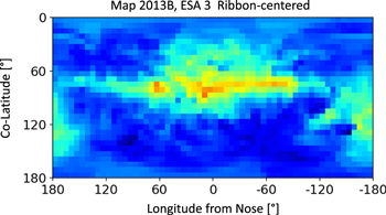
Figure A1. Ribbon-centered ENA flux from map 2013B, ESA 3 (∼1.11 keV passband). The ribbon center is located at the "north pole" of the map, and the ribbon itself appears as a constant latitude feature at ∼75° colatitude. The heliospheric nose (upwind direction) is located at (0°, 48°) in this projection. Also present is a roughly circular flux enhancement centered on the nose and overlapping with the ribbon due to compression of the upwind HS. Another flux maximum centered at 180° longitude and approximately 120° colatitude calls out the tail direction.
Download figure:
Standard image High-resolution imageAs mentioned in Section 2.1, this study makes use of 6 month ENA sky maps so as to achieve the highest time resolution possible for application of the sounding method (the maps are also CG- and survival probability–corrected). This presents a challenge for ribbon separation because the marginal statistics in a single 6 month map can make it difficult to distinguish the ribbon flux from the GDF. In fact, for this reason, previous authors (e.g., Schwadron et al. 2011; Dayeh et al. 2019) carried out ribbon separation by summing together multiple maps. We overcome this issue by averaging in longitude every 24° of pixels (4 pixels), resulting in 15 longitude strips across the sky, each with 30 6° wide bins in latitude spanning pole-to-pole. When performing ribbon separations on 6 month intervals, the use of CG-corrected maps makes sense; otherwise, transforming a spacecraft-frame map to a ribbon-centered frame would mix ribbon observations made in the Ram and anti-Ram directions, which would have the result of mixing very different flux levels.
We now describe the separation procedure and refer the reader to Figure A2. For each longitude strip, we identify a set of bins on either side of the ribbon (but not including the ribbon) and fit a second-order polynomial (a parabola) to the ENA flux to capture the shape of the GDF beneath the ribbon. For the lowest four energy steps (ESAs 2–5), the fit region spans 90° of latitude but excludes the 40° wide region between 55° and 95° latitude (measured from the north pole) where we expect contributions from the ribbon. For the top energy step (ESA 6), the ribbon appears to be somewhat wider, so the parabola fit region spans 100°, where we exclude the 50° wide region between 50° and 100°.
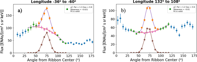
Figure A2. (a) Longitudinal strip of average ENA fluxes between longitudes −60° and −36° for map 2013B, ESA 3, showing a valid partitioning of flux between the GDF and the ribbon. For this strip, the ribbon is superimposed on a flux enhancement centered on the nose (see Figure A1). Green points are fit by a second-order polynomial (parabola); orange points are fit by a Gaussian after the parabola fit is removed. Based on the ratio of the Gaussian fit to the Gaussian + parabola fits, the original flux is partitioned between the GDF (pink points) and the ribbon (brown points). The blue points are not included in the analysis. Note that the legend reports the reduced χ2 for the parabola and Gaussian fits and the skewness of the ribbon. (b) Longitudinal strip averaging fluxes between longitudes 108° and 132 In this case, the parabola fit is concave-up, consistent with a depression of flux within the heliospheric lobes.
Download figure:
Standard image High-resolution imageThe choice of a second-order polynomial to fit the GDF was based on the following considerations. Certainly, a higher-order fit than first-order (linear) is warranted. As seen in Figures 2(a) and (b), the curvature observed outside the ribbon is likely to continue naturally beneath the ribbon. For example, in Figure A2(a), the GDF fit is associated with a flux enhancement at the nose, which is likely to maintain a similar shape across the ribbon. On the other hand, using a higher-than-second-order fit is not well justified. From heliospheric models, it is not expected that the GDF will show much resolvable small-scale structure in ENA maps; indeed, in the regions of the sky outside the ribbon, IBEX ENA maps show little evidence of structure on scales less than ∼45 Furthermore, it would be difficult to fit real higher-order structure considering the limited number of bins (eight or so) included in the GDF fit. In developing the separation method, higher-order fits (up to fourth order) were explored, but they were abandoned because of the tendency of the fits to be dominated by statistical fluctuations. Note that our separation method does not remove higher-order structure. The separated GDF and ribbon flux maps will share any of the original structure between them, weighted by the relative amount of flux attributed to the ribbon versus the GDF.
For the entire fit region, we subtract flux from each pixel dictated by the polynomial fit, and then we fit a symmetric Gaussian to what remains, capturing the ribbon flux. The choice of a Gaussian is entirely empirical, but this has been commonly employed (e.g., Schwadron et al. 2011; Funsten et al. 2013; Dayeh et al. 2019). Fitting an asymmetric Gaussian was also considered, but after subtraction of the parabola, the skewness of the remaining flux was analyzed, and it was determined that in the vast majority of cases, the skewness values indicate a highly symmetric distribution for the ribbon. That is, most of the apparent asymmetry observed in cuts across the ribbon in total ENA maps can be attributed to the shape of the underlying GDF.
Once the Gaussian fit is made, the total flux in each of the original 6° × 6° pixels of the ribbon-centered map is partitioned into GDF and ribbon flux by taking the ratio of the Gaussian fit to the total Gaussian-plus-polynomial fit to arrive at the fraction of flux to associate with the ribbon versus the GDF (see Figure A2(a)). For example, suppose the total flux in a pixel is 120 (cm2 s sr keV)−1, the polynomial fit gives a flux of 68 (cm2 s sr keV)−1, and the Gaussian fit gives a flux of 47 (cm2 s sr keV)−1. Then,  of the total flux, or 49.1 (cm2 s sr keV)−1, is assigned to the ribbon, and the remaining 70.9 (cm2 s sr keV)−1 is assigned to the GDF. Note that this method conserves flux. The fits are just used to assign the relative amounts of flux in a given pixel to one structure or the other.
Although the ribbon is usually a very strong feature in the sky, at certain longitudes, it is sometimes fairly weak or the statistics are poor, such that it is hard to cleanly fit the ribbon. Therefore, we place certain bounds on the fits, and when these are exceeded, the fit is thrown out and the strip is left unaltered. The following requirements are imposed in order for a fit to be considered valid.
- 1.The location of the Gaussian fit peak must be within the expected bounds for the peak ribbon flux. For ESAs 2–5, the peak of the Gaussian fit must be between 65° and 85° latitude (in the ribbon-centered frame), or approximately within ±10° of the nominal ribbon opening angle of 748. For ESA 6, the range is broader, 60°–90°, because the ribbon appears somewhat wider there.
- 2.The width of the Gaussian must be within the range identified for the ribbon width. The standard deviation of the Gaussian fit must be between σ = 4° and 15° (4° and 18° for ESA 6). This corresponds to an FWHM for the ribbon fit between 10° and 38° (10° and 46° for ESA 6). If the fit is wider than this, it usually means that no ribbon is detectable and the routine is trying to fit a Gaussian to the GDF. If the fit is narrower than this, it means that there is no detectable ribbon but statistical fluctuations cause 1 or 2 pixels to be significantly higher than their neighbors.
- 3.The peak of the Gaussian must be larger than twice the measured flux uncertainty averaged over the four bins nearest the peak. In other words, the peak must be statistically significant.
The values for these bounds were tuned by trial and error, and in the vast majority of cases, they allow for accurate identification of the ribbon (or its absence) and quantification of its properties. Figure A3 shows two cases of invalid fits.

Figure A3. Two examples of invalid fits. The longitude range indicated at the top is relative to the nose. Panel (a) is from map 2014B, ESA 2, and panel (b) is from map 2013B, ESA 3. The fit in panel (a) is invalid because the Gaussian fit is too narrow (σ ∼ <∼4°) to be considered a ribbon. It is also invalidated because the size of the peak is comparable to the statistical uncertainty and thus considered inconclusive. In panel (b), the Gaussian fit peaks outside the expected range of latitudes for the ribbon peak (between 65° and 85°). In this case, the Gaussian fit is picking up the edge of the enhanced flux coming from the downwind direction at mid-energies in the heliospheric tail (McComas et al. 2013).
Download figure:
Standard image High-resolution imageOnce the ribbon/GDF partition fractions are determined, they are applied to the original 6° × 6° pixels that comprise the 24° wide longitude-averaged strips. Thus, two ribbon-centered frame maps are created, one of the GDF and one of the ribbon flux, examples of which are shown in Figure A4, derived from the total ENA flux map in Figure A1. These maps are then transformed to create ecliptic-frame GDF and ribbon maps (see Figure 1). Looking at the GDF map in Figure A4, one would be hard-pressed to identify the presence of any residual ribbon features. This is not to say that there is not some over- or undersubtraction of ribbon flux. In fact, there most likely is, since (a) the fits are based on 24° longitude-averaged strips, whereas the partitioning is applied to individual 6° × 6° pixels, and (b) we use a purely empirical model for the shape of the ribbon, and until we have a better theoretical understanding of its structure, we are certain to make separation errors.
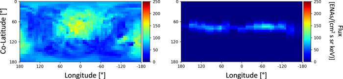
Figure A4. Ribbon-centered GDF (left) and ribbon (right) ENA maps for map 2013B, ESA 3. Compare to the total sky map shown in Figure A1. See Figure 1 for the ecliptic-frame versions.
Download figure:
Standard image High-resolution image
In the ribbon maps in Figure A4 and Figure 1, there are occasional gaps along the ribbon that indicate portions where the fit was invalidated. Often, these occur around 135° ecliptic longitude due to the poor statistics associated with interference from the Earth's magnetosphere being in the foreground. Gaps also occur with increasing frequency at higher energies. Looking at the original maps in Figure 1 (left column), one can see that this is due to the fact that the ribbon becomes weaker relative to the GDF and even appears to break up into segments. The gaps are probably larger than they need to be due to the longitude averaging that is necessary for applying the separation procedure to 6 month maps. If it is desired to more accurately separate the ribbon without longitude averaging but at the expense of time resolution, one can average together multiple maps to improve statistics and carry out ribbon separation on 6° wide strips, as has been done previously by other authors (e.g., Schwadron et al. 2011; Dayeh et al. 2019).